Transfer learning is a game-changer in the realm of computer vision, enabling us to solve complex tasks even with limited datasets. By leveraging pre-trained models, we can either extract valuable features or fine-tune them for specific applications. This guide takes you step-by-step through the fundamentals and practical implementation of transfer learning in computer vision.
Understanding Transfer Learning
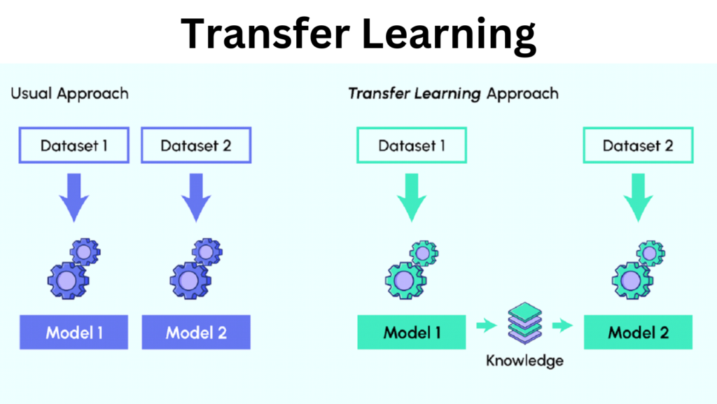
Transfer learning uses a model trained on a large dataset (e.g., ImageNet) as a foundation for solving new tasks. The pre-trained model can either:
Act as a Feature Extractor: Extract features from the pre-trained model and add a custom classifier for the new task.
Be Fine-Tuned: Modify the pre-trained model’s weights by continuing training on the new dataset.
Why Use Transfer Learning?
Transfer learning provides several benefits:
Reduces Training Time: Saves computational resources by reusing pre-trained models.
Requires Less Data: Works effectively with smaller datasets.
Improves Performance: Leverages robust feature extraction for better generalization.
Pre-Requisites
To follow along, you need:
Libraries: Python, TensorFlow/Keras, or PyTorch.
Basic Knowledge: Neural networks, convolutional neural networks (CNNs).
Hands-On with TensorFlow/Keras
In this example, we’ll use transfer learning for a binary image classification task.
Step 1: Load a Pre-Trained Model
from tensorflow.keras.applications import VGG16
# Load the pre-trained model without the top classification layer
base_model = VGG16(weights=’imagenet’, include_top=False, input_shape=(224, 224, 3)
Step 2: Freeze the Pre-Trained Layers
Freezing prevents the pre-trained weights from being updated during training.
for layer in base_model.layers:
layer.trainable = False
Step 3: Add Custom Layers
Build a custom classifier tailored to the task.
from tensorflow.keras import layers, models
model = models.Sequential([
base_model,
layers.Flatten(),
layers.Dense(128, activation=’relu’),
layers.Dropout(0.5),
layers.Dense(1, activation=’sigmoid’) # Binary classification
])
Step 4: Compile the Model
Define the optimizer, loss function, and evaluation metrics.
model.compile(optimizer=’adam’, loss=’binary_crossentropy’, metrics=[‘accuracy’])
Step 5: Prepare the Dataset
Use ImageDataGenerator for data preprocessing and augmentation.
from tensorflow.keras.preprocessing.image import ImageDataGenerator
train_datagen = ImageDataGenerator(
rescale=1./255, rotation_range=20, zoom_range=0.2, horizontal_flip=True
)
train_generator = train_datagen.flow_from_directory(
‘path_to_train_data’,
target_size=(224, 224),
batch_size=32,
class_mode=’binary’
)
Step 6: Train the Model
history = model.fit(train_generator, epochs=10, steps_per_epoch=100)
Step 7: Fine-Tune the Model
Unfreeze some layers of the pre-trained model and retrain.
for layer in base_model.layers[-4:]: # Unfreeze the last 4 layers
layer.trainable = True
model.compile(optimizer=’adam’, loss=’binary_crossentropy’, metrics=[‘accuracy’])
history_fine = model.fit(train_generator, epochs=5, steps_per_epoch=100)
Hands-On with PyTorch
Let’s solve a binary classification task for ants and bees using PyTorch.
Step 1: Load Data
Preprocess the data using torchvision.transforms.
from torchvision import datasets, transforms
# Data augmentation and normalization
data_transforms = {
‘train’: transforms.Compose([
transforms.RandomResizedCrop(224),
transforms.RandomHorizontalFlip(),
transforms.ToTensor(),
transforms.Normalize([0.485, 0.456, 0.406], [0.229, 0.224, 0.225])
]),
‘val’: transforms.Compose([
transforms.Resize(256),
transforms.CenterCrop(224),
transforms.ToTensor(),
transforms.Normalize([0.485, 0.456, 0.406], [0.229, 0.224, 0.225])
]),
}
# Load datasets
data_dir = ‘data/hymenoptera_data’
image_datasets = {x: datasets.ImageFolder(os.path.join(data_dir, x), data_transforms[x])
for x in [‘train’, ‘val’]}
Step 2: Load a Pre-Trained Model
We’ll use ResNet18 for this example.
from torchvision import models
model_ft = models.resnet18(weights=’IMAGENET1K_V1′)
num_ftrs = model_ft.fc.in_features
model_ft.fc = nn.Linear(num_ftrs, 2) # Adjust for binary classification
Step 3: Train and Evaluate
Define a training loop to fine-tune the model.
from torch.optim import lr_scheduler
import torch.optim as optim
criterion = nn.CrossEntropyLoss()
optimizer_ft = optim.SGD(model_ft.parameters(), lr=0.001, momentum=0.9)
scheduler = lr_scheduler.StepLR(optimizer_ft, step_size=7, gamma=0.1)
# Training loop
def train_model(model, dataloaders, criterion, optimizer, scheduler, num_epochs=25):
for epoch in range(num_epochs):
for phase in [‘train’, ‘val’]:
if phase == ‘train’:
model.train()
else:
model.eval()
running_loss = 0.0
running_corrects = 0
for inputs, labels in dataloaders[phase]:
inputs, labels = inputs.to(device), labels.to(device)
optimizer.zero_grad()
with torch.set_grad_enabled(phase == ‘train’):
outputs = model(inputs)
_, preds = torch.max(outputs, 1)
loss = criterion(outputs, labels)
if phase == ‘train’:
loss.backward()
optimizer.step()
running_loss += loss.item() * inputs.size(0)
running_corrects += torch.sum(preds == labels.data)
if phase == ‘train’:
scheduler.step()
Key Considerations
Dataset Size: Feature extraction is ideal for small datasets, while fine-tuning works better with larger datasets.
Pre-Trained Models: Experiment with models like ResNet, EfficientNet, and MobileNet.
Data Augmentation: Enhances generalization by diversifying training data
Next Steps
Extend transfer learning to multi-class classification.
Explore domains like object detection or semantic segmentation.
Fine-tune hyperparameters for better performance.
Transfer learning simplifies complex computer vision tasks and opens up opportunities for innovation. Start experimenting today and unlock its potential!