Principal Component Analysis (PCA) is one of the most widely used techniques in machine learning and statistics for dimensionality reduction. Whether you are working on feature selection, data visualization, or noise reduction, PCA simplifies complex datasets into manageable dimensions while retaining essential information. At the heart of PCA are two mathematical concepts: eigenvalues and eigenvectors. In this blog, we’ll explore how eigenvalues and eigenvectors form the foundation of PCA, making it a powerful tool for data analysis.
What is PCA?
Principal Component Analysis is a statistical method used to transform high-dimensional data into a lower-dimensional format. It does so by identifying the directions in which the data varies the most, called principal components. These components allow us to:
Reduce Dimensionality: Lower the number of variables while preserving most of the dataset’s variance.
Simplify Data: Make datasets easier to visualize and analyze.
Enhance Performance: Improve the efficiency of machine learning models by reducing noise and redundancy.
PCA works by transforming the data into a new coordinate system defined by the principal components. These components are determined by the eigenvalues and eigenvectors of the dataset’s covariance matrix.
How PCA Uses Eigenvalues and Eigenvectors
To understand PCA, it’s essential to delve into the roles of eigenvalues and eigenvectors. Let’s break this down step by step.
Step 1: Computing the Covariance Matrix
The first step in PCA is to calculate the covariance matrix of the dataset. This matrix measures how much each pair of variables in the dataset varies together. It provides a mathematical representation of the relationships between the features.
Step 2: Eigendecomposition of the Covariance Matrix
Once the covariance matrix is computed, PCA performs eigendecomposition, a process that breaks down the matrix into its eigenvalues and eigenvectors. These are the key to identifying the principal components:
-
Eigenvectors represent the directions (or axes) in the data space where the variance is maximum.
-
Eigenvalues quantify the magnitude of variance captured by each eigenvector.
Understanding Eigenvalues
What Are Eigenvalues?
Eigenvalues are scalar values that indicate the amount of variance captured by their corresponding eigenvectors. In simpler terms, they tell us how much of the data’s variability is explained by each principal component.
Why Are Eigenvalues Important?
Ranking Principal Components: Eigenvalues allow us to rank the principal components by importance. Components with higher eigenvalues capture more variance and are thus more significant.
Dimensionality Reduction: By focusing on the eigenvectors with the largest eigenvalues, we can reduce the dataset’s dimensions while retaining most of its information.
Variance Explained: Eigenvalues help us calculate the proportion of the total variance explained by each principal component. This is crucial for determining how many components to keep.
Example:
Imagine a dataset with three features (x, y, z). After applying PCA, we find three eigenvalues: 5, 3, and 1. These values indicate that the first principal component explains the most variance (5 units), followed by the second (3 units), and the third (1 unit). To reduce dimensionality, we might keep only the first two components, capturing 80% of the total variance.
Understanding Eigenvectors
What Are Eigenvectors?
Eigenvectors are special vectors that remain unchanged in direction when a linear transformation (like PCA) is applied. In PCA, eigenvectors represent the axes of the new coordinate system, known as principal components.
Why Are Eigenvectors Important?
Principal Directions: Eigenvectors define the directions in which the data varies the most. Each eigenvector corresponds to a principal component.
Feature Contribution: Eigenvectors show how much each original feature contributes to the principal component. This helps us understand the structure of the data.
Data Transformation: The original data is projected onto the eigenvectors to create the new, lower-dimensional representation.
Example:
For a dataset with two features, the eigenvectors might point in directions that are linear combinations of the original features (e.g., “x + y” or “x – y”). These directions represent the principal components that capture the most variance in the data.
The PCA Process: A Step-by-Step Guide
Here’s how PCA utilizes eigenvalues and eigenvectors to transform your data:
Step 1: Standardize the Data
Before applying PCA, standardize the dataset to have a mean of zero and unit variance. This ensures that all features contribute equally to the analysis.
Step 2: Compute the Covariance Matrix
Calculate the covariance matrix to capture the relationships between features.
Step 3: Perform Eigendecomposition
Decompose the covariance matrix into its eigenvalues and eigenvectors.
Step 4: Select Principal Components
Sort the eigenvalues in descending order and select the top eigenvectors corresponding to the largest eigenvalues. These eigenvectors form the principal components.
Step 5: Project the Data
Transform the original data by projecting it onto the selected principal components. This creates a new dataset with reduced dimensions.
Visualizing Eigenvalues and Eigenvectors
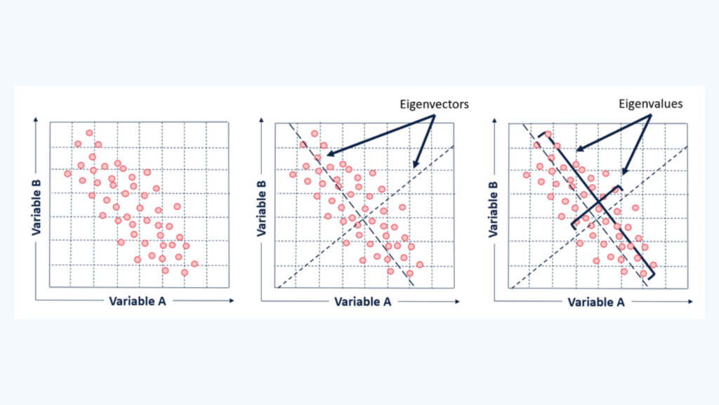
To better understand the role of eigenvalues and eigenvectors, imagine a 2D scatter plot of data points:
The eigenvectors are lines (axes) pointing in the directions of maximum variance.
The eigenvalues determine the length of these lines, indicating how much variance is captured along each axis.
In this way, the eigenvectors define the new coordinate system, and the eigenvalues show the importance of each axis.
Benefits of Using PCA
1. Dimensionality Reduction
PCA simplifies datasets by reducing the number of features while preserving the most significant information. This is particularly useful for:
High-dimensional datasets where many features are correlated.
Improving computational efficiency in machine learning algorithms.
2. Noise Reduction
By focusing on components with high eigenvalues, PCA filters out noise and less important features, leading to cleaner data.
3. Visualization
PCA enables the visualization of high-dimensional data by projecting it into 2D or 3D spaces.
4. Feature Engineering
Principal components can serve as new features, capturing the essence of the original dataset.
Key Takeaways
Eigenvalues and eigenvectors are the foundation of PCA. They help identify the principal components, which are the directions of maximum variance in the data.
Eigenvalues quantify the variance captured by each component, while eigenvectors define the directions.
PCA reduces dimensionality, enhances interpretability, and improves the efficiency of data analysis.
By understanding how PCA leverages eigenvalues and eigenvectors, you can unlock the full potential of your data. Whether you’re a data scientist, machine learning enthusiast, or researcher, mastering PCA is a crucial step toward effective data analysis.